Hitting the Ground Running
This post assumes you’ve already read part 1 and part 2 for “Individual Athlete Monitoring in R.” If you haven’t I’d suggest you go back to part 2 for some context for this post. Otherwise, you’re going to be pretty lost. Let’s go.
It’s Predicting Time
Last time, we built a linear mixed model with the lme4 package called final model. This model used two categorical fixed effects (season, phase within season) along with five grand mean centered numeric fixed effects (total distance, work rate, hi-speed running distance, time spent in drills, and total practice duration) to predict log transformed rpetl values. We further included athletes nested within season as random intercept effects in the model to reflect that we’re analyzing repeated-measures data where the magnitudes of the relationships between variables may differ between athletes and between seasons. I know that’s a bit of a mouthful, so seriously, go back and look at part 2 if you’re not sure what I’m talking about. The model output is below.
## Linear mixed model fit by maximum likelihood  ['lmerMod']
## Formula: log.rpetl ~ (1 | season/athlete) + odometer + work.rate + hi.run +
##     field.minutes + duration + season + phase
##    Data: rpe.scaled
##
##      AIC      BIC   logLik deviance df.resid
##   2460.7   2550.4  -1215.3   2430.7     2915
##
## Scaled residuals:
##     Min      1Q  Median      3Q     Max
## -5.9599 -0.6227  0.0843  0.6488  3.9842
##
## Random effects:
##  Groups         Name        Variance Std.Dev.
##  athlete:season (Intercept) 0.02931  0.1712
##  season         (Intercept) 0.00000  0.0000
##  Residual                   0.12566  0.3545
## Number of obs: 2930, groups:  athlete:season, 103; season, 4
##
## Fixed effects:
##                 Estimate Std. Error t value
## (Intercept)      5.29222    0.03815 138.709
## odometer         0.04029    0.03012   1.338
## work.rate        0.20622    0.02180   9.459
## hi.run           0.03150    0.01170   2.691
## field.minutes    0.06492    0.02000   3.246
## duration         0.31320    0.01110  28.217
## seasonFall 2015 -0.17880    0.04960  -3.605
## seasonFall 2016 -0.40376    0.05327  -7.579
## seasonFall 2017 -0.47707    0.05711  -8.354
## phaseNC          0.07035    0.01740   4.043
## phasePOST        0.02321    0.02188   1.060
## phasePRE         0.32283    0.02331  13.848
##
## Correlation of Fixed Effects:
##             (Intr) odomtr wrk.rt hi.run fld.mn duratn sF2015 sF2016 sF2017
## odometer    -0.035
## work.rate    0.033 -0.886
## hi.run       0.032 -0.420  0.120
## field.mints  0.022 -0.816  0.782  0.193
## duration     0.071 -0.155  0.122 -0.047 -0.257
## sesnFll2015 -0.706  0.001 -0.004  0.007 -0.007  0.002
## sesnFll2016 -0.646 -0.014  0.001  0.026  0.005  0.018  0.510
## sesnFll2017 -0.610  0.001  0.002  0.005 -0.005  0.003  0.476  0.443
## phaseNC     -0.261  0.062 -0.090 -0.060 -0.026 -0.210 -0.007 -0.047 -0.018
## phasePOST   -0.167  0.079 -0.083 -0.162  0.016 -0.129 -0.052 -0.043 -0.035
## phasePRE    -0.212  0.122 -0.107 -0.114 -0.078 -0.242  0.000 -0.032 -0.012
##             phasNC phPOST
## odometer
## work.rate
## hi.run
## field.mints
## duration
## sesnFll2015
## sesnFll2016
## sesnFll2017
## phaseNC
## phasePOST    0.474
## phasePRE     0.522  0.366
## convergence code: 0
## boundary (singular) fit: see ?isSingular
Under normal circumstances, you would probably be comparing several methods to model the relationship between external load metrics and rpetl. In that case, you would go through a cross-validation process similar to [1], where you split your data into training and test sets to determine which method is most effective in predicting previously-unseen data. We’ll leave that for some other time, though. For now, let’s attempt to tackle a real-life problem: using our model, can we identify anomalous rpetl values? I’m going to split the data so that we’re attempting to predict rpetl values for the final three weeks of the 2017 season. I’ll also re-create the model based on this trimmed dataset.
# Create a training set
training.data <- rpe.scaled[date < "2017-10-16"]

prediction.data <- rpe.scaled[date >= "2017-10-16"]

# New model based on training.data
final.model <- lmer(log.rpetl ~ (1|season/athlete) + odometer + work.rate + hi.run +
                         field.minutes + duration + season + phase,
                       data = training.data, REML = FALSE)
## boundary (singular) fit: see ?isSingularIt’s important to note the scaled predictors in training.data aren’t quite correct because the original scaling process included the data from prediction.data. In the real world, your training data will lag behind the data you want to predict by a few days or a few weeks. The amount of lag is up to you as I haven’t found any satisfying answers in reading about predictive modeling. You could easily set up a script that would update your training dataset every few days to keep your model up-to-date. You could, however, base prediction.data’s scaled coefficients on the entire dataset to ensure the scaled values accurately reflect the data. Anyway, let’s start by using our model to predict rpetl values for training.data. Remember, we log transformed rpetl last time, so we’ll need to back-transform the predictions via exp().
# Predict log-transformed rpetl values from our final model
training.data$log.prediction <- predict(final.model, training.data)

# Back-transform the predictions to raw rpetl values
training.data[, prediction := exp(log.prediction)]

knitr::kable(training.data[1:10, c("athlete", "date", "rpetl", "prediction")])| athlete | date | rpetl | prediction |
|---|---|---|---|
| Jonathan Sanchez | 2014-08-13 | 450 | 592.1312 |
| Dhaki al-Naim | 2014-08-13 | 450 | 623.3140 |
| Corey Klocker | 2014-08-13 | 450 | 578.5048 |
| Issac Martinez | 2014-08-13 | 450 | 418.6855 |
| Phoenix Lee | 2014-08-13 | 360 | 470.6439 |
| Carroll Bond | 2014-08-13 | 540 | 598.4328 |
| Neulyn Whyte | 2014-08-13 | 720 | 684.5372 |
| Jonathan Sanchez | 2014-08-14 | 450 | 335.1269 |
| Bobby Landry | 2014-08-14 | 270 | 351.3422 |
| Daniel Thompson | 2014-08-14 | 270 | 309.3395 |
Notice the predictions aren’t spot-on. We can quantify our model’s prediction error at both the group level and individual level. Model error is typically reported as mean absolute error (MAE) or root mean square error (RMSE). [3] recommend using a combination of the between-subject and within-subject RMSE (a.k.a. root mean square deviation) to set limits and confidence intervals for truly anomalous prediction errors. A drawback to RMSE is that it penalizes outliers more heavily compared to MAE. Since we’re interested in identifying outliers in this case, we might examine the MAE instead. But in the words of the Old El Paso commercial, “Por que no los dos?” We can examine both approaches pretty easily with the caret package.
# Group RMSE
training.data[, .(group.RMSE = RMSE(prediction, rpetl))]
## group.RMSE
## 1: 72.43846# Individual RMSE
training.data[, .(individual.RMSE = RMSE(prediction, rpetl)), by = athlete]## athlete individual.RMSE
## 1: Jonathan Sanchez 79.65152
## 2: Dhaki al-Naim 98.24133
## 3: Corey Klocker 66.35323
## 4: Issac Martinez 71.24416
## 5: Phoenix Lee 96.51796
## 6: Carroll Bond 84.44877
## 7: Neulyn Whyte 73.54454
## 8: Bobby Landry 69.01649
## 9: Daniel Thompson 74.79385
## 10: Ethan Phouminh 61.53159
## 11: Brandon Mclaughlin 82.08851
## 12: Henry Douglas 57.64887
## 13: Brandon Tan 54.92733
## 14: Laten Absher 58.61063
## 15: John Mowers 68.33314
## 16: Jeremy Pribbenow 90.63118
## 17: Leo Ortiz 61.26317
## 18: Richard Bruff 99.38963
## 19: Naseer el-Saladin 63.81937
## 20: Zackarie Broeren 63.17699
## 21: Erik Dores 87.85881
## 22: Fawzi al-Shaheed 99.88159
## 23: Joseph Johnston 68.37198
## 24: Mashal el-Tahir 84.34851
## 25: Blake Graybill 117.84725
## 26: Nicholas Rayas Coronado 63.69189
## 27: Augustus Gallo 82.49120
## 28: Tammaam al-Sheikh 78.90438
## 29: Sadi el-Hamady 55.18857
## 30: Zachary Nestor 64.08365
## 31: Amru el-Zia 47.99908
## 32: Dominik Gibson 73.62863
## 33: Sung-Jin Le 93.70942
## 34: Tyrone Teka 88.54565
## 35: Carlos Vasquez 58.78742
## 36: Benjamin Beverly 63.96766
## 37: Tyler Choo 44.67102
## 38: Calvin Charlie 74.99400
## 39: Braden Bliler 69.91302
## 40: Quentin Mooney 64.44706
## 41: Bakar el-Burki 61.10722
## 42: Dan Munoz 50.43102
## 43: Matthew Futamata 103.58369
## 44: Isaac Conway 84.91036
## 45: Nicholas Mckay 69.71548
## 46: Scottie Salaz 57.65266
## 47: Magnus Yang 58.41908
## 48: Muaaid el-Kamel 67.63561
## 49: Ruben Ayala 47.00549
## 50: Jordan Hughes 63.20713
## 51: Cuauhtemoc Box 67.61856
## 52: Yusri al-Abdoo 62.40452
## 53: Ron Quintana 63.10565
## 54: Samuel Llanas Brito 33.69042
## athlete individual.RMSE# Group MAE
training.data[, .(group.MAE = MAE(prediction, rpetl))]## group.MAE
## 1: 50.79352# Individual MAE
training.data[, .(individual.MAE = MAE(prediction, rpetl)), by = athlete]## athlete individual.MAE
## 1: Jonathan Sanchez 57.57782
## 2: Dhaki al-Naim 68.45952
## 3: Corey Klocker 47.82331
## 4: Issac Martinez 54.65807
## 5: Phoenix Lee 69.40985
## 6: Carroll Bond 63.20898
## 7: Neulyn Whyte 56.20448
## 8: Bobby Landry 50.03018
## 9: Daniel Thompson 56.23135
## 10: Ethan Phouminh 47.88505
## 11: Brandon Mclaughlin 60.74419
## 12: Henry Douglas 41.67811
## 13: Brandon Tan 45.46249
## 14: Laten Absher 47.92199
## 15: John Mowers 50.86440
## 16: Jeremy Pribbenow 60.24945
## 17: Leo Ortiz 43.53623
## 18: Richard Bruff 72.82061
## 19: Naseer el-Saladin 52.18722
## 20: Zackarie Broeren 42.95711
## 21: Erik Dores 56.30851
## 22: Fawzi al-Shaheed 62.52946
## 23: Joseph Johnston 48.36695
## 24: Mashal el-Tahir 58.73721
## 25: Blake Graybill 80.55885
## 26: Nicholas Rayas Coronado 43.80600
## 27: Augustus Gallo 58.77337
## 28: Tammaam al-Sheikh 64.73494
## 29: Sadi el-Hamady 40.39463
## 30: Zachary Nestor 50.79137
## 31: Amru el-Zia 33.30804
## 32: Dominik Gibson 53.35034
## 33: Sung-Jin Le 59.76749
## 34: Tyrone Teka 60.98581
## 35: Carlos Vasquez 45.81151
## 36: Benjamin Beverly 44.98752
## 37: Tyler Choo 34.61203
## 38: Calvin Charlie 60.85675
## 39: Braden Bliler 52.30069
## 40: Quentin Mooney 50.99086
## 41: Bakar el-Burki 51.60180
## 42: Dan Munoz 43.30896
## 43: Matthew Futamata 72.77470
## 44: Isaac Conway 51.32585
## 45: Nicholas Mckay 52.86036
## 46: Scottie Salaz 42.19793
## 47: Magnus Yang 39.66141
## 48: Muaaid el-Kamel 55.96923
## 49: Ruben Ayala 30.08009
## 50: Jordan Hughes 55.71311
## 51: Cuauhtemoc Box 48.89419
## 52: Yusri al-Abdoo 41.74455
## 53: Ron Quintana 42.21368
## 54: Samuel Llanas Brito 25.39538
## athlete individual.MAEIt’s pretty interesting to examine the spread of the prediction errors among athletes. I would wager we could improve the model’s predictive accuracy by accounting for pre-training wellness, previous match outcome, injury status, MD minus, and other contextual factors, but I think a RMSE of ~ 72 units (range 33 - 118) and MAE of 51 units (range 25 - 81) will be acceptable for today’s example. Further, an approach similar to [2], where anomalous points produced by sickness and injury are retroactively removed, might be another way to improve the model’s predictive ability. Unfortunately, we didn’t collect contextual data like that, so we’re stuck with what we have.
Identifying Anomalies
First, let’s add our between- and within-subject RMSE and MAE to prediction.data.
# Group RMSE
group.RMSE <- training.data[, RMSE(prediction, rpetl)]

# Individual RMSE
individual.RMSE <- training.data[, .(individual.RMSE = RMSE(prediction, rpetl)),
                             by = athlete]

# Group MAE
group.MAE <- training.data[, MAE(prediction, rpetl)]

# Individual MAE
individual.MAE <- training.data[, .(individual.MAE = MAE(prediction, rpetl)),
                                by = athlete]

# Add model predictions to prediction.data
prediction.data$log.prediction <- predict(final.model, prediction.data)

prediction.data[, prediction := exp(log.prediction)]

# Add group MAE and RMSE to prediction.data
prediction.data[, ":=" (prediction.error = rpetl - prediction,
                        group.RMSE = group.RMSE,
                        group.MAE = group.MAE)]

# Add individual RMSE and MAE via merge()
prediction.data <- merge(prediction.data, individual.RMSE, sort = FALSE)

prediction.data <- merge(prediction.data, individual.MAE, sort = FALSE)
Once we’ve added the RMSE and MAE to prediction.data, we can visualize them.
# RMSE plot
ggplot(prediction.data, aes(x = date, y = prediction.error)) +
  geom_pointrange(aes(ymin = prediction.error - individual.RMSE,
                      ymax = prediction.error + individual.RMSE)) +
  geom_ribbon(aes(ymin = -group.RMSE,
                  ymax = group.RMSE), alpha = 0.2) +
  theme_bw() + facet_wrap(~athlete, scales = "free_y") +
  labs(title = "Predictions vs. Actual (RMSE)",
       x = "Date",
       y = "Actual - Predicted RPETL (AU)") +
  geom_hline(aes(yintercept = 0), linetype = "dotdash")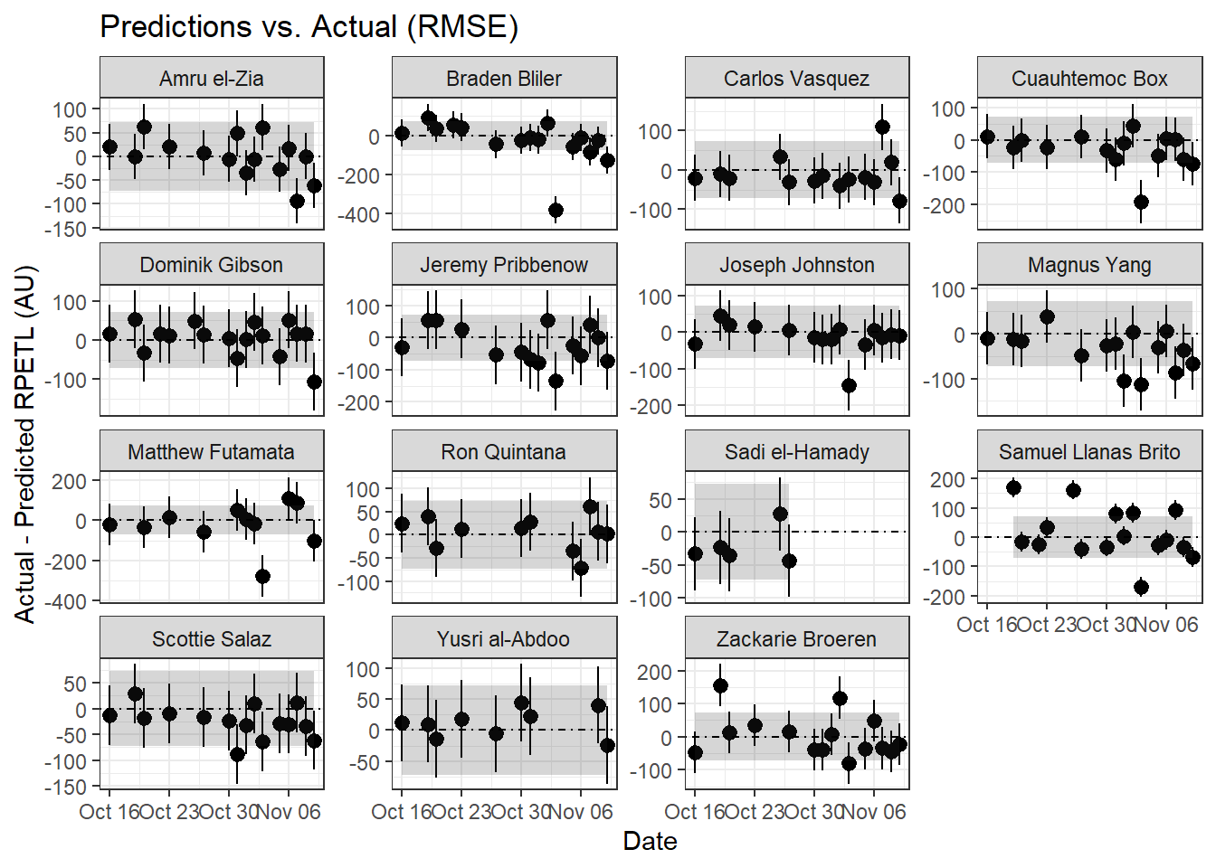
# MAE plot
ggplot(prediction.data, aes(x = date, y = prediction.error)) +
  geom_pointrange(aes(ymin = prediction.error - individual.MAE,
                      ymax = prediction.error + individual.MAE)) +
  geom_ribbon(aes(ymin = -group.MAE,
                  ymax = group.MAE), alpha = 0.2) +
  theme_bw() + facet_wrap(~athlete, scales = "free_y") +
  labs(title = "Predictions vs. Actual (MAE)",
       x = "Date",
       y = "Actual - Predicted RPETL (AU)") +
  geom_hline(aes(yintercept = 0), linetype = "dotdash")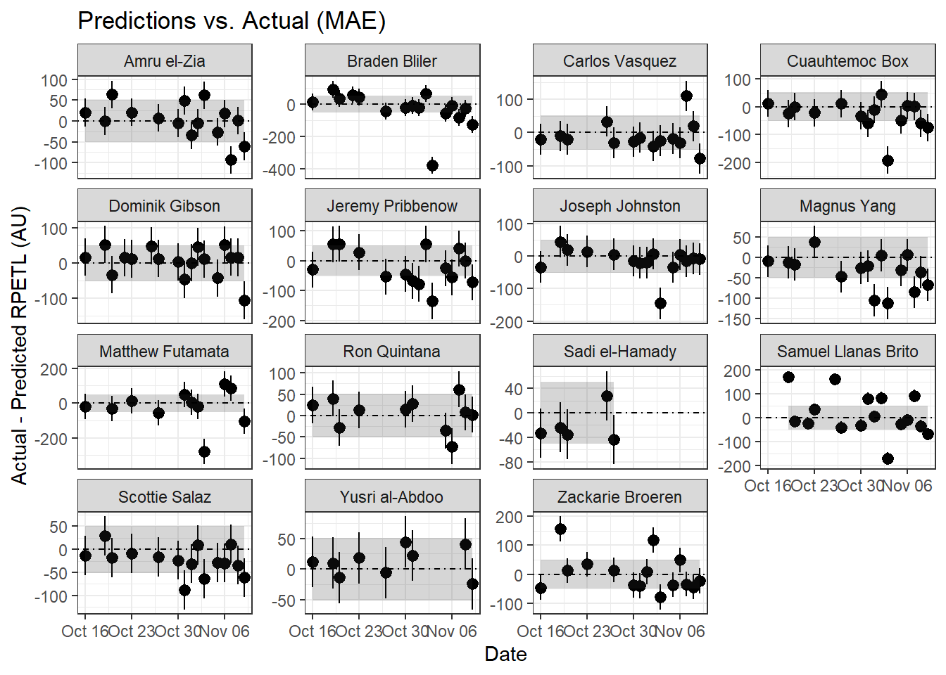
It’s pretty difficult to make out what’s happening at the group level, so let’s zoom in on a single athlete (Samuel Llanas Brito).
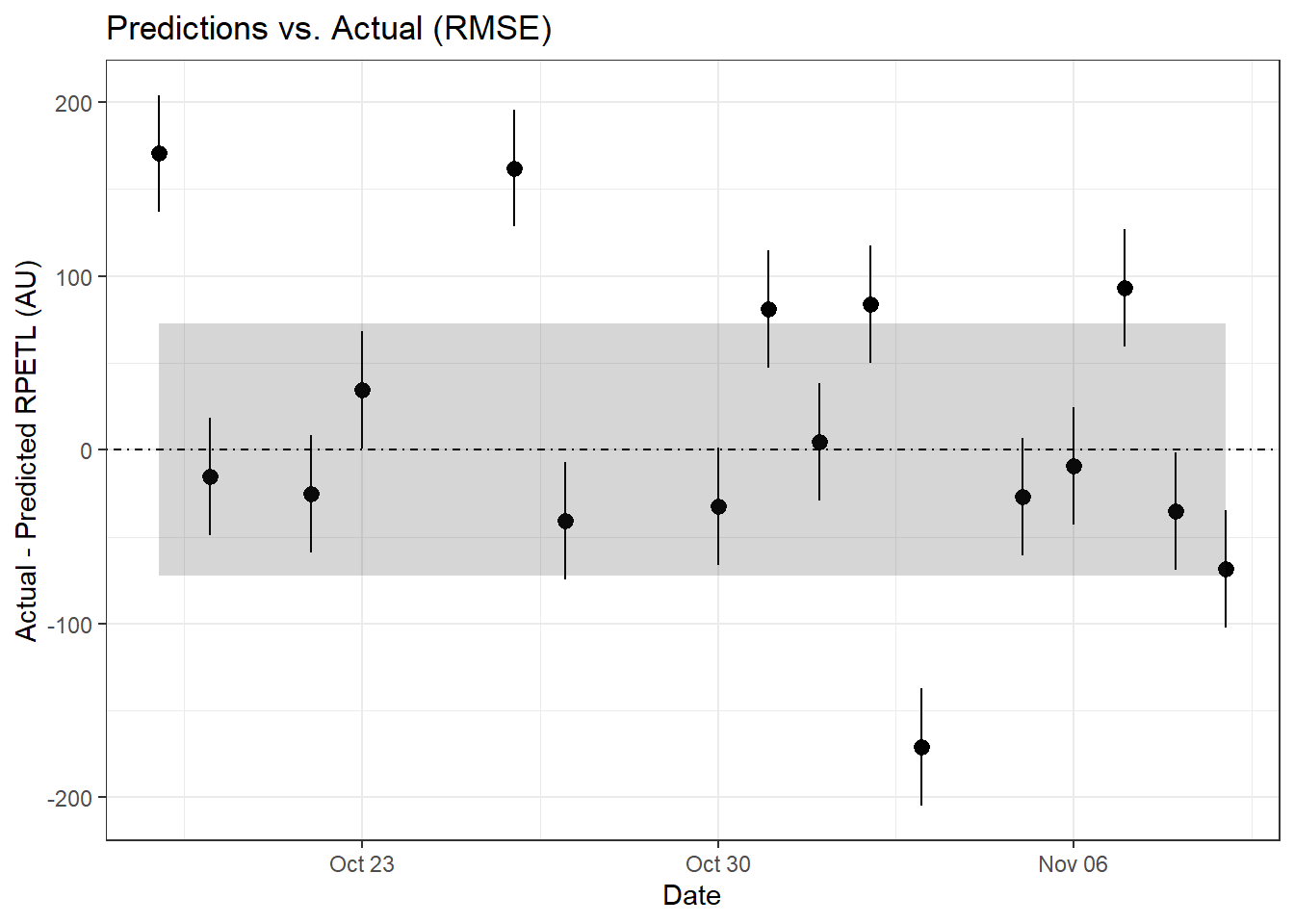
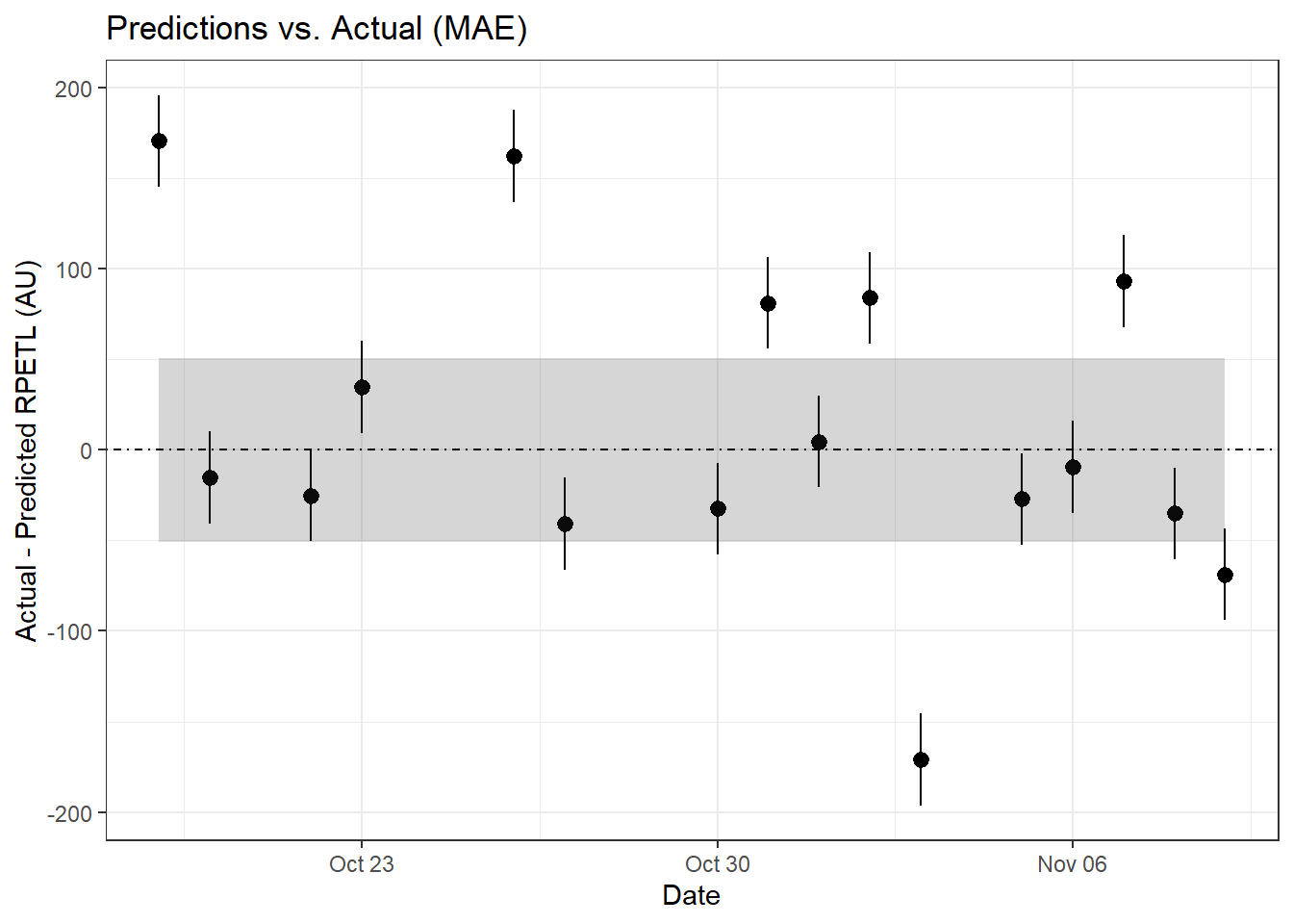
For Samuel, both the RMSE and MAE methods are in relative agreement with two sessions drastically above predicted, three sessions just above the error limits, and one session well below what was predicted. Having access to the original data, I can tell you the first anomalous point comes from the athlete’s first practice back from a contact injury sustained 9 days before. It’s safe to assume that contributed to the anomalous score. Similarly, the second point came after his first match involvement following his injury. We can assume some lingering match fatigue may have contributed, which is also likely reflected in his above-prediction scores on Oct. 31st and Nov. 2nd. For him, an altered training setup (bike/pool fitness, play as a neutral, etc.) with more gradual RTP may have been preferrable to immediate full involvement. Of course, it’s easy to say that now, but examining this data retroactively can also help us understand how we can improve our RTP process in the future.
As for the extreme over-prediction on November 3rd, that was an intrasquad during a bye week. Having been with the team through a number of these over the years, late-season intrasquads tended to be more laid back and ended with a low-stakes round of penalty kicks where the athletes inentionally attempted to distract the athlete taking the PK. The relaxed atmosphere and extended low-intensity (and sometimes silly) round of PKs probably contributed to the lower-than-predicted rpetl values. And if you look back at the other athletes’ data, you’ll notice a similar trend for most of the team. Again, situations like this are where adding additional complexity to the model (percent of practice time spent in drills, maybe? Feel free to experiment.) may improve its predictive power.
Wrapping Up

I think this is a good place to stop. Hopefully parts 2 and 3 have given you a decent introduction to using mixed model predictions as part of your athlete monitoring. This post wasn’t comprehensive, by any means, and probably left out some parts of the process. So if you’re still a little unsure of where to go from here, feel free to hit me up on Twitter or via email and I’ll get back to you ASAP. Also, I know I didn’t address using the fixed effects’ coefficients for athletes with limited data; if you would like to see my thoughts on how to implement that, let me know and I’ll add an addendum to this post. Finally, feel free to share your own ideas on how to improve the predictive accuracy of the model. I always love hearing others’ ideas!
1 Carey DL, Ong K, Morris ME, Crow J, Crossley KM. Predicting ratings of perceived exertion in australian football players: Methods for live estimation. International Journal of Computer Science in Sport 2016; 15: 64–77 Available from: https://doi.org/10.1515/ijcss-2016-0005
2 Vandewiele G, Geurkink Y, Lievens M, Ongenae F, Turck FD, Boone J. Enabling training personalization by predicting the session rate of perceived exertion (sRPE). 2017;
3 Ward P, Coutts AJ, Pruna R, McCall A. Putting the “i” back in team. International Journal of Sports Physiology and Performance 2018; 1–14 Available from: https://doi.org/10.1123/ijspp.2018-0154